“Better code, better life. ”
前言
这周工作室没开会,so今天有时间再更一篇
本篇主要看了matplotlib的柱状图的画法和一些numpy的函数的使用问题
最后会又一个实践,画出了全市场的pe分布图
正文
点击使用Jupyter nbviewer查看代码
1. 首先是最基本的柱状图的画法
import numpy as np
import pandas as pd
import matplotlib.mlab as mlab
import matplotlib.pyplot as plt
np.random.seed(0)
num_bins = 50
mu = 100
sigma = 15
x = mu + sigma * np.random.randn(500)
#np.random.rand(n) 产生标准正态分布, 即均值为0 标准差为1 的高斯分布 扥同于 np.random.normal(0, 1, n)
# x = mu + sigma * np.random.randn(500) 是产生500个均值为100, 方差为15 的随机数
# 等于 x = np.random.normal(100, 15, 500)
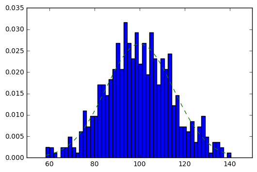
fig, ax = plt.subplots()
n, bins, patches = ax.hist(x, num_bins, normed=1)
#这里ax.hist()即是画柱状图的函数
#x 为数据,num_bins为分隔的段数
plt.show()

2. 这里就展现了python各种库的数据处理能力的强大之处
y = mlab.normpdf(bins, mu, sigma)
#这里用mlab.normpdf()方法来给柱状图拟合了一个正态分布曲线
ax.plot(bins, y, '--')
fig
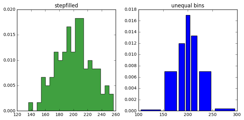
3. 下面介绍另外两种柱状图 stepfilled 和 bar 类型
np.random.seed(0)

mu = 200
sigma = 25
x = np.random.normal(mu, sigma, size=100)

fig, (ax0, ax1) = plt.subplots(ncols=2, figsize=(8, 4))
#这里的ncols 参数即是字表的列数
ax0.hist(x, 20, normed=1, histtype='stepfilled', facecolor='g', alpha=0.75)
ax0.set_title('stepfilled')
#这里的ax0是的histtype 为setpfilled即每个数段的柱状图是连续的
#第二个参数20 是分的段数
# Create a histogram by providing the bin edges (unequally spaced).
bins = [100, 150, 180, 195, 205, 220, 250, 300]
ax1.hist(x, bins, normed=1, histtype='bar', rwidth=0.8)
#这里的histtype是 bar类型即是每个bar独立分隔,便于观看
#其中bins 这个参数是一个List,即按list中给出的数来分段
ax1.set_title('unequal bins')

fig.tight_layout()
plt.show()
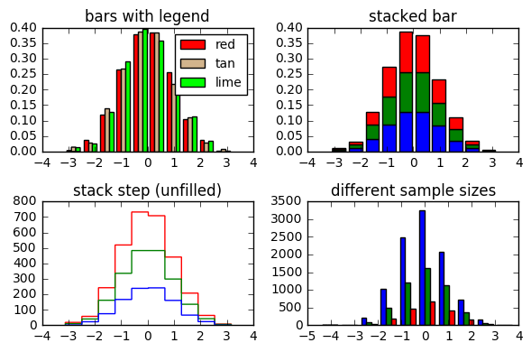
4. 接着是多组数据展示在同一张表上的对比情况图
np.random.seed(0)

n_bins = 10
x = np.random.randn(1000, 3)
#产生了一个1000*3的矩阵,每一列都是一千个正态分布的随机数
fig, axes = plt.subplots(nrows=2, ncols=2)
ax0, ax1, ax2, ax3 = axes.flatten()

colors = ['red', 'tan', 'lime']
ax0.hist(x, n_bins, normed=1, histtype='bar', color=colors, label=colors)
ax0.legend(prop={'size': 10})
ax0.set_title('bars with legend')
#第一种类型是legend 主要可以用来横向对比不同组别数据的分布,在每一个区段占比的多少
ax1.hist(x, n_bins, normed=1, histtype='bar', stacked=True)
ax1.set_title('stacked bar')
#第二种类型是纵向对比,显示总体数据的分布,并且总体数据每个分段的柱状图上用颜色来区分不同组别数据的占比
ax2.hist(x, n_bins, histtype='step', stacked=True, fill=False)
ax2.set_title('stack step (unfilled)')
#第三种类型是第二种的一个变形,请参考上面一个lab
# Make a multiple-histogram of data-sets with different length.
x_multi = [np.random.randn(n) for n in [10000, 5000, 2000]]
ax3.hist(x_multi, n_bins, histtype='bar')
ax3.set_title('different sample sizes')
#第四种类型换了一种原始数据,x_multi是一个list,里面x[0]是一个10000个数据的正态分布随机数,x[1],x[2]分别是5000,2000个正态分布的随机数
#第四种显示了每个分段不同数据的个数
fig.tight_layout()
plt.show()
5. 常用的柱状图类型学习完毕,下面开始实践画出全市场股票的pe分布图
点击下载pe数据
df = pd.read_csv('pe_tatio.csv')
df = pd.DataFrame([df['code'], df['pe_ratio']]).T
df.head(5)
#首先读取数据,读到的df如下
| code | pe_ratio | |
|---|---|---|
| 0 | 300372.XSHE | -4.49 |
| 1 | 300656.XSHE | 28.86 |
| 2 | 603269.XSHG | 37.14 |
| 3 | 300653.XSHE | 39.47 |
| 4 | 002873.XSHE | 30.23 |
#接着对df进行处理,分为沪市,深市,创业板分别统计
def fun(x):
    if x[0][0] == '3':
        return 'gem'
    elif x[0][0] == '6':
        return 'sh'
    else :
        return 'sz'

df['type'] = df.apply(fun, axis=1)
df.head(5)
| code | pe_ratio | type | |
|---|---|---|---|
| 0 | 300372.XSHE | -4.49 | gem |
| 1 | 300656.XSHE | 28.86 | gem |
| 2 | 603269.XSHG | 37.14 | sh |
| 3 | 300653.XSHE | 39.47 | gem |
| 4 | 002873.XSHE | 30.23 | sz |
gem = df[df['type']=='gem']
sh = df[df['type']=='sh']
sz = df[df['type']=='sz']
gem.head(5)
| code | pe_ratio | type | |
|---|---|---|---|
| 0 | 300372.XSHE | -4.49 | gem |
| 1 | 300656.XSHE | 28.86 | gem |
| 3 | 300653.XSHE | 39.47 | gem |
| 5 | 300029.XSHE | -37.67 | gem |
| 6 | 300649.XSHE | 82.49 | gem |
df.groupby('type').describe()
#使用describe方法可以大概查看一下分类后的信息的一些参数
| code | pe_ratio | ||
|---|---|---|---|
| type | |||
| gem | count | 639 | 639.00 |
| unique | 639 | 623.00 | |
| top | 300331.XSHE | 66.10 | |
| freq | 1 | 2.00 | |
| sh | count | 1273 | 1273.00 |
| unique | 1273 | 1218.00 | |
| top | 601991.XSHG | 44.19 | |
| freq | 1 | 3.00 | |
| sz | count | 1323 | 1323.00 |
| unique | 1323 | 1256.00 | |
| top | 002007.XSHE | 26.13 | |
| freq | 1 | 3.00 |
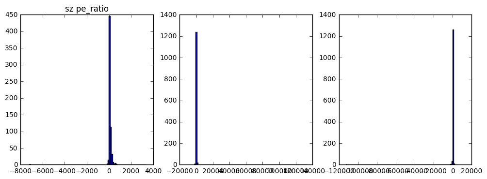
开始绘图,不过从结果来看有点不理想,主要是由于数据的极值问题,还需对原始数据进一步处理
#下面开始用今天能学到的新东西绘制柱状图啦
fig, (ax0, ax1, ax2) = plt.subplots(ncols=3, figsize=(12, 4))
gem_pe = gem['pe_ratio'].values
sh_pe = sh['pe_ratio'].values
sz_pe = sz['pe_ratio'].values

n_bins = 100

ax0.hist(gem_pe, n_bins)
ax0.set_title('gem pe_ratio')

ax1.hist(sh_pe, n_bins)
ax0.set_title('sh pe_ratio')

ax2.hist(sz_pe, n_bins)
ax0.set_title('sz pe_ratio')
plt.show()
这里用了标准的去极值方法,即把原始数据中大于 mean + 3 * std 的数据用 mean + 3 * std 代替,小于 mean - 3 * std 的数据用 mean - 3 * std 代替
def altertremum(array):
    sigma = array.std()
    mu = array.mean()
    array[array > mu + 3*sigma] = mu + 3*sigma
    array[array < mu - 3*sigma] = mu - 3*sigma
    return array

fig, (ax0, ax1, ax2) = plt.subplots(ncols=3, figsize=(12, 4))
gem_pe = gem['pe_ratio'].values
sh_pe = sh['pe_ratio'].values
sz_pe = sz['pe_ratio'].values

n_bins = 50

gem_pe = altertremum(gem_pe)
sh_pe = altertremum(sh_pe)
sz_pe = altertremum(sz_pe)

ax0.hist(gem_pe, n_bins)
ax0.set_title('gem pe_ratio')

ax1.hist(sh_pe, n_bins)
ax1.set_title('sh pe_ratio')

ax2.hist(sz_pe, n_bins)
ax2.set_title('sz pe_ratio')
plt.show()
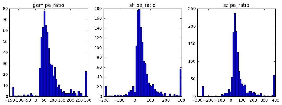
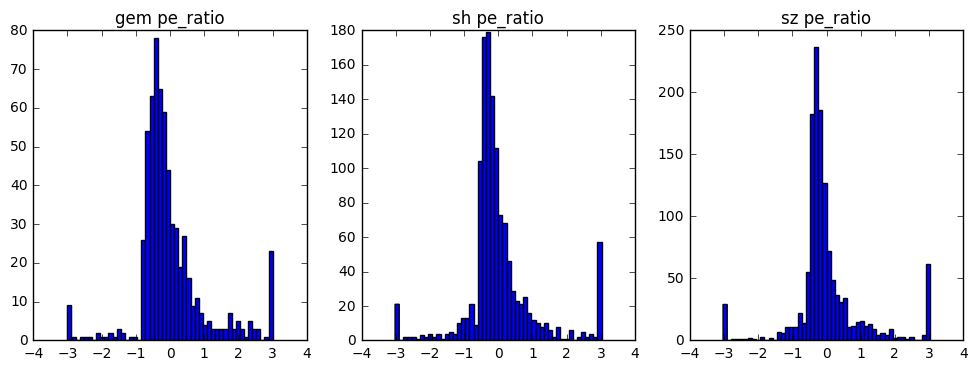
经过去极值处理的数据已经有了一定的区分度了,下面进行数据标准化处理(此步骤对pe数据来说完全没有意义!!仅为了实践处理方法)
'''
1.求出各变量(指标)的算术平均值(数学期望)xi和标准差si ;
2.进行标准化处理:
zij=(xij-xi)/si
其中:zij为标准化后的变量值;xij为实际变量值。
3.将逆指标前的正负号对调。
'''
def neutralize(array):
    mu = array.mean()
    std = array.std()
    array = (array - mu)/std
    return array


fig, (ax0, ax1, ax2) = plt.subplots(ncols=3, figsize=(12, 4))
gem_pe = gem['pe_ratio'].values
sh_pe = sh['pe_ratio'].values
sz_pe = sz['pe_ratio'].values

n_bins = 50

gem_pe = neutralize(gem_pe)
sh_pe = neutralize(sh_pe)
sz_pe = neutralize(sz_pe)

ax0.hist(gem_pe, n_bins)
ax0.set_title('gem pe_ratio')

ax1.hist(sh_pe, n_bins)
ax1.set_title('sh pe_ratio')

ax2.hist(sz_pe, n_bins)
ax2.set_title('sz pe_ratio')
plt.show()
后记
今天自代码写完到post的时间可比昨天快多了。。。
—— Simon 于2017.5